
From blinking to absorption: how one molecule becomes a spectrum
1. Two pictures of the same molecule
A confocal microscope focused on a dilute dye film records a trace of light that comes in bursts: bright intervals separated by dark gaps, never two photons at the same instant, with occasional long blackouts when the molecule shelves into a triplet state. The same dye dissolved at micromolar concentration in a cuvette gives a smooth UV–visible band on a spectrometer, a continuous curve peaked at some wavelength and broadened over tens of nanometers. The two experiments are looking at the same electronic transition, but the first sees events and the second sees a rate.
The question this note answers is how one picture becomes the other. The route runs through a single object — the molecular Jablonski diagram — read at different scales. One molecule absorbs and emits one photon at a time, so its spectrum is a sequence of discrete events governed by the radiative lifetime. A bulk sample contains enough molecules that the individual events blur into a steady current, and the envelope of that current is the absorption band. The same diagram, taken to higher order in the light–matter interaction, also describes two-photon absorption: the nonlinear signal is the same transition accessed with two photons instead of one.
2. One molecule: absorption and emission as discrete events
Start with one molecule and two electronic states: a ground state \(|g\rangle\) and an excited state \(|e\rangle\) separated by \(E_{eg} = \hbar\omega_{eg}\). In a weak light field the molecule behaves like a two-level system. Absorption promotes it from \(|g\rangle\) to \(|e\rangle\) at a rate \(k_{\text{abs}} = \sigma \Phi\), where \(\sigma\) is the absorption cross section and \(\Phi\) is the photon flux. Once in \(|e\rangle\) it waits for a time of order \(1/k_{\text{rad}}\) and then emits one photon, dropping back to \(|g\rangle\) (Figure 1).
The spontaneous emission rate is not an independent parameter: it is fixed by the same transition dipole moment \(|\boldsymbol{\mu}_{eg}|\) that sets the absorption cross section. That connection is the Einstein \(A\) coefficient, and it is why a strong absorber is also a fast emitter.1,2 For the single molecule, though, the important point is that the cycle is quantized: it absorbs one photon, then emits one photon, then waits to absorb another. Within the two-level model there is no state above \(|e\rangle\) to absorb into, so the molecule cannot take up a second photon of the same energy while it is excited. A real dye does have higher electronic states and can show excited-state absorption, but at the weak intensities considered here that channel is negligible, and the emission stream stays intermittent at the single-photon level.
Figure 1. One molecule’s Jablonski diagram. Absorption promotes the molecule from \(|g\rangle\) to \(|e\rangle\); spontaneous emission returns it. A triplet state \(|t\rangle\) acts as a dark shelf, producing the long dark intervals in a single-molecule trace.
3. Why a single molecule blinks
The intermittency has two signatures. The first is antibunching: the probability of detecting two photons at essentially the same instant drops to zero, because the molecule must be re-excited before it can emit again — an effect measured directly on a single dye molecule in a solid.3 The second is the longer dark intervals produced by triplet shelving, spectral diffusion, or photobleaching.4 In those dark periods the molecule is no longer in the \(|g\rangle \leftrightarrow |e\rangle\) cycle at all; it has been diverted to a non-emissive state or has changed its resonance out of the excitation window.
Consequently the spectrum of a single molecule is not a continuous band. It is a sequence of \(\delta\)-like emission events, each centred at the molecule’s own transition frequency, separated by waiting times drawn from the absorption and emission rates. Only when enough of these events are collected does the histogram of detected photons start to look like a line shape, and even then it is the line shape of one molecule in one local environment.
4. From one molecule to many: ensemble averaging
Now put \(N\) copies of the molecule in the beam, dilute enough that each interacts with the light independently. The total absorption rate is simply \(N\) times the single-molecule rate, and that proportionality is the content of the Beer–Lambert law: the fraction of light absorbed in a thin slab is the number of molecules in the slab times the single-molecule cross section.5
Two kinds of broadening separate the ensemble band from the single-molecule line. The finite lifetime of \(|e\rangle\) gives every molecule the same homogeneous Lorentzian line shape of half-width \(\gamma\),
\[L(\nu;\nu_i) = \frac{\gamma/\pi}{(\nu-\nu_i)^2 + \gamma^2},\]
centred at that molecule’s own transition frequency \(\nu_i\). But no two molecules sit in identical surroundings — local strain, polarity, and packing shift each \(\nu_i\) slightly — so across the ensemble the centre frequencies are scattered. Modelling that scatter as a Gaussian distribution of standard deviation \(\sigma\) and averaging the Lorentzians,
\[S_N(\nu) = \frac{1}{N}\sum_{i=1}^{N} L(\nu;\nu_i),\]
turns the forest of narrow lines into a single smooth, inhomogeneously broadened envelope as \(N\) grows (Figure 2).6
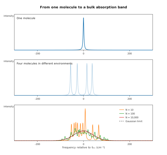
Figure 2. From one molecule to a bulk band. Top: a single two-level molecule has a narrow Lorentzian line. Middle: four molecules in slightly different environments give four shifted Lorentzians. Bottom: averaging over ensembles of \(N\) molecules recovers the smooth, inhomogeneously broadened band measured in a cuvette; the dashed curve is the analytic Gaussian limit.
Code 1 is the demonstration behind Figure 2, condensed to its two moves: draw each molecule’s centre frequency from a Gaussian, then average the Lorentzians. It uses only the Python standard library.
Code 1. The core of the ensemble-averaging demonstration: each molecule contributes the same Lorentzian cross section shifted to its own centre frequency, and the ensemble spectrum is the plain average.
import math, random

def lorentzian(x, x0, gamma):
    return (gamma / math.pi) / ((x - x0) ** 2 + gamma ** 2)

gamma = 2.0              # homogeneous linewidth (HWHM), cm^-1
sigma = 40.0             # inhomogeneous Gaussian width, cm^-1
N = 10_000

random.seed(0)
centres = [random.gauss(0.0, sigma) for _ in range(N)]

nu = [-300 + 600 * i / 999 for i in range(1000)]
spectrum = [sum(lorentzian(x, c, gamma) for c in centres) / N for x in nu]
On the plotted grid the one-molecule line has a full width at half maximum of 4.1 cm⁻¹, while the averaged band of the \(N = 10{,}000\) ensemble is 94.6 cm⁻¹ wide — within 0.4% of the analytic Gaussian limit \(2\sqrt{2\ln 2}\,\sigma\) = 94.2 cm⁻¹. The sum is not mysterious: each term is the same microscopic cross section, only shifted by the local environment. A spectrometer does not resolve the individual terms; it measures their average.
5. The bulk absorption spectrum is the same transition dipole
The integrated intensity of the bulk absorption band is proportional to \(|\boldsymbol{\mu}_{eg}|^2\), exactly the same quantity that sets the single-molecule emission rate.7 The molar absorptivity post traced this in the other direction: measuring an absorption spectrum is a way of measuring a lifetime, because both observables read the same transition dipole.
What changes in the bulk measurement is not the molecule but the bookkeeping. A continuous absorption curve does not mean one molecule is absorbing continuously; it means the ensemble is absorbing at a steady rate. The cross section \(\sigma(\nu)\) is still a per-molecule quantity. Beer–Lambert’s law, \(A = \varepsilon(\nu)\,c\,\ell\), merely multiplies that per-molecule response by the number of molecules in the beam. The smoothness comes from the large \(N\) limit, not from any change in the microscopic physics.
6. The nonlinear extension: two-photon absorption from the same diagram
The same Jablonski diagram that governs one-photon absorption also governs nonlinear absorption, read at second order in the field. In one-photon absorption a single photon of energy \(\hbar\omega_{eg}\) carries the molecule from \(|g\rangle\) to \(|e\rangle\). In two-photon absorption the molecule reaches the same state by taking up two photons whose energies sum to \(E_{eg}\) — in the degenerate case drawn in Figure 3, two photons of \(\hbar\omega_{eg}/2\) each — passing through a virtual intermediate state that is not a stationary state of the molecule.8
Figure 3. The same two states read at first and second order. One-photon absorption (red) reaches \(|e\rangle\) with a single photon. Two-photon absorption (green) reaches the same state with two photons of half the energy, passing through a virtual intermediate level that is not a stationary state of the molecule.
The selection rules of the two routes are complementary rather than shared. In a centrosymmetric molecule, where every electronic state has a definite parity, a one-photon transition connects states of opposite parity (\(g \leftrightarrow u\)), while a two-photon transition connects states of the same parity (\(g \leftrightarrow g\) or \(u \leftrightarrow u\)) — each photon contributes one parity flip.9 The selection-rules post works through where those rules come from; in a molecule without an inversion centre neither rule is strict, and the same excited state can be reachable by both routes with different strengths. The nonlinear signal is also weak: its rate scales with the square of the intensity, which is why two-photon absorption matters only under a focused laser. But it is the same molecule, the same pair of states, and the same transition dipoles, read at higher order.
7. Reproducibility of the demonstrations
Figures 1 and 3 are TikZ energy-level diagrams compiled by the site build.
Figure 2 and the linewidths quoted in §4 are generated by
research/from-blinking-to-absorption/src/ensemble_broadening.py — Python
3.12.3, standard library only, seeded with random.seed(0) so every run is
bit-reproducible — of which Code 1 is a condensed excerpt. Running
python3 research/from-blinking-to-absorption/src/ensemble_broadening.py from
the repository root rewrites the figure and the canonical
results/summary.json, from which generate-metrics.mjs derives the values
cited in the text; the experiment directory records the environment and
publishes every file involved.
8. Where the model stops
Everything above assumes independent molecules. The single-molecule/bulk connection breaks down when intermolecular interactions matter — excitonic coupling, aggregation, concentrated dyes — because the ensemble spectrum then stops being a sum of one-molecule spectra. The two-photon treatment is perturbative: strong fields bring saturation and Rabi oscillations, which need a different model, and the two-level approximation itself hides the higher excited states responsible for excited-state absorption. Finally, the clean split between one homogeneous linewidth and one inhomogeneous distribution is an idealization: a single molecule’s resonance can wander in time (spectral diffusion), so which broadening counts as “the molecule’s own” depends on the timescale of the measurement.
9. Summary
The single-molecule trace and the bulk absorption band are not two different phenomena; they are the same Jablonski diagram read at different scales. One molecule emits photons one at a time, with waiting times set by the absorption flux and the radiative lifetime. An ensemble of many molecules, each in a slightly different environment, averages those discrete lines into the smooth band a spectrometer records. The cross section that governs the single-molecule absorption rate is the same cross section that appears in Beer–Lambert’s law; the only new ingredient in the bulk measurement is the number of molecules.
The nonlinear extension is the same diagram read at higher order. Two-photon absorption reaches \(|e\rangle\) with two photons that share the transition energy, through a virtual state, and in centrosymmetric molecules its selection rules are complementary to those of one-photon absorption. Underneath all three versions — blinking, bulk absorption, and nonlinear absorption — is the same transition dipole.