
Extending Villatoro et al.'s SIREN benchmark: the momentum recovery region
Abstract
Villatoro, Geraci, and Schiavazzi’s 2026 article, Assessing the Performance of Correlation-Based Multi-Fidelity Neural Emulators, benchmarks SIREN networks on multi-fidelity tasks and writes down one of the two circulating SIREN parameterizations.1,2 This post is an independent extension of that benchmark — the fourth in a series that reimplements the written K1 specification in NumPy and probes how the two parameterizations train — and it measures something the series left open: as the heavy-ball momentum coefficient \(\beta\) varies over \(\{0, 0.3, 0.6, 0.9, 0.99\}\), how wide is the set of learning rates at which the described convention reaches the official convention’s error floor?
The answer is not a monotone widening. The stage-1 recovery counts are 0, 0, 0, 1, and 12 grid points in order of increasing \(\beta\): nothing below \(\beta=0.9\), a knife-edge of 0.03 decades at \(\beta=0.9\) hard against the divergence boundary, and a wide low-rate plateau of at least 0.68 decades at \(\beta=0.99\) — while the divergence boundary, which had tracked the heavy-ball \(1+\beta\) prediction within a grid step through \(\beta=0.9\), collapses back to its plain-SGD value (1.000 relative to \(\beta=0\)) and an instability band with finite errors as large as 7.55×10⁷¹ opens below it. The registered hypothesis — monotone widening, with recovery at every \(\beta>0.5\) — is falsified: \(\beta=0.6\) recovers at no tested rate.
Introduction
The two SIREN parameterizations represent the same function at initialization and train differently. The described convention draws hidden weights from \(\mathcal{U}(\pm\sqrt{6/n})\) and applies \(\sin(Wx+b)\); the official implementation draws from \(\mathcal{U}(\pm\sqrt{6/n}/\omega_0)\) and applies \(\sin(\omega_0(Wx+b))\).2,3 On the K1 task of Villatoro et al., this series has measured the convention gap under Adam, under plain SGD, and under heavy-ball momentum at \(\beta=0.9\). That last note found the gap closed at exactly one tested learning rate — the final stable point of a \(0.05\)-decade grid, one grid step below the divergence boundary — with the boundary itself moved up by a factor consistent with the quadratic heavy-ball bound \(2(1+\beta)/L\), against \(2/L\) for gradient descent.
One tested point is a measurement of a set’s size only in the coarsest sense. If the recovered-rate region scales with the gap between the heavy-ball and gradient-descent stability bounds, it should close as \(\beta\to0\) and widen toward \(1+\beta\) — the reading the momentum-control note’s Conclusion queued as its next experiment. Whether it does is what this note measures. A region that widens smoothly with \(\beta\) would make momentum a usable repair for the described convention; a region that stays a single grid point, or vanishes at intermediate \(\beta\), would make the \(\beta=0.9\) recovery a knife-edge.
Hypothesis. The recovery region widens monotonically (nondecreasing) with \(\beta\in\{0, 0.3, 0.6, 0.9, 0.99\}\), riding the stability boundary upward, and the described convention reaches the official error floor at at least one tested rate for every \(\beta>0.5\). Falsifier, fixed before running: the width does not vary monotonically with \(\beta\), or the described convention reaches the floor at no tested rate for some \(\beta>0.5\). Either outcome was publishable: the first names a usable repair, the second a knife-edge, and both are rules a practitioner can act on. The hypothesis, falsifier, grids, recovery rule, and decision rule were frozen in a preregistration before the canonical run, and are reported as registered.
Computational Methods
All numbers were produced on CPython 3.13.12, arm64 macOS 26.5.2, NumPy 2.4.4, no other result dependency; the figure additionally used matplotlib 3.11.1. This was a computer-only numerical experiment using synthetic inputs and deterministic code; it involved no living subjects and no human or animal data. Model, task, data, seeds, and manual backprop are those of the momentum-control note without change, vendored from its committed script into this experiment’s sweep driver with unused code paths removed: K1 from Villatoro et al., eq. (4), fit by their multi-fidelity architecture with the exact low-fidelity function, the nonlinear branch a SIREN of three hidden layers of sixteen units, \(\omega_0=30\), \(c=6\), \(N_H=32\) Sobol’ samples plus the two boundary points, errors reported as normalized test MSE.1 Both conventions in a repetition start from one parameter draw, with the matched official parameterization dividing hidden weights and biases by \(\omega_0\) — the same declared idealization as before; the official repository rescales weights alone.2,3 The update is full-batch heavy-ball momentum, \(v \leftarrow \beta v + g\), \(\theta \leftarrow \theta - \text{lr}\cdot v\), for \(20{,}000\) epochs; \(\beta=0\) through the same code path is the plain-SGD control. The vendored training path was checked against the earlier script on this machine before the canonical run: identical output, bit for bit, on the July recovery cell. The earlier notes ran on a different machine (CPython 3.10.12, aarch64 Linux, NumPy 2.2.6); values that sit at the float64 error floor move at roundoff scale across environments, so floor values quoted here are this environment’s, while the recovery events and divergence boundaries reproduce the earlier notes’ values exactly.
I used neither the source authors’ program nor their data: their code remains unreleased, K1 is a closed-form test case printed in the paper, and every number describes my independent NumPy reimplementation of their written specification.
The frozen protocol has two stages. Stage 1 runs both conventions at each \(\beta\in\{0, 0.3, 0.6, 0.9, 0.99\}\) on a common \(35\)-point grid from \(10^{-4}\) to \(10^{-2.3}\) at \(0.05\)-decade spacing, three repetitions (data seeds \(1544\)–\(1546\), parameter seeds \(7000\)–\(7002\) as before) — 1050 trainings. A grid point counts as recovered when the median normalized test MSE over the three repetitions is at most \(10^{-24}\), a threshold frozen about three orders of magnitude above the official convention’s \(\beta=0.9\) floor; a repetition that returns a non-finite error makes its point not recovered rather than being excluded. Stage 2 applies a frozen refinement rule: for each \(\beta\) with at least one recovered stage-1 point, a \(0.01\)-decade grid from \(0.10\) decades below the lowest recovered rate up to the lowest rate at which any repetition diverged, 672 further trainings. The decision rule: supported if the stage-1 recovered counts are nondecreasing in \(\beta\) and every \(\beta\in\{0.6, 0.9, 0.99\}\) recovers at at least one tested rate; falsified otherwise; inconclusive had the counts been equal with the refined widths unable to separate them. Recovery counts at the sensitivity thresholds \(10^{-20}\) and \(10^{-28}\) are recorded alongside. Code 1 gives the exact commands; the canonical outputs are stage1.json and stage2.json, and every result number in this post resolves from the committed metrics projection at build time.
Code 1. Exact commands for the canonical run and the metrics projection, from the repository root and experiment directory respectively.
cd research/momentum-recovery-region
python3 src/run_sweep.py    # stage 1, then stage 2 by the frozen rule
node generate-metrics.mjs   # project results/*.json into metrics.json
Results
Table 1 summarizes stage 1. The described convention’s recovered-point counts across \(\beta\in\{0, 0.3, 0.6, 0.9, 0.99\}\) are 0, 0, 0, 1, 12; the counts are identical at the \(10^{-20}\) and \(10^{-28}\) sensitivity thresholds. The best described median test error is \(10^{-5}\) to \(10^{-6}\) at \(\beta\le0.6\), 2.03×10⁻²⁹ at \(\beta=0.9\), and 7.58×10⁻³¹ at \(\beta=0.99\). The official convention’s median test error over finite grid points decreases from 8.70×10⁻⁷ at \(\beta=0\) to 5.78×10⁻³⁰ at \(\beta=0.99\).
Table 1. Stage-1 results per momentum coefficient: described-convention recovered-point count at the frozen \(10^{-24}\) threshold, best tested learning rate and best median normalized test MSE, official-convention median over finite points, first divergent learning rate, and the divergence boundary relative to \(\beta=0\) against the \(1+\beta\) prediction.
| \(\beta\) | recovered points | best tested lr | best described MSE | official median MSE | first divergent lr | boundary ratio | \(1+\beta\) |
|---|---|---|---|---|---|---|---|
| \(0\) | 0 | 6.3096×10⁻⁴ | 2.72×10⁻⁵ | 8.70×10⁻⁷ | 7.0795×10⁻⁴ | 1.000 | \(1\) |
| \(0.3\) | 0 | 7.9433×10⁻⁴ | 7.70×10⁻⁶ | 1.28×10⁻¹⁰ | 1.0000×10⁻³ | 1.413 | \(1.3\) |
| \(0.6\) | 0 | 1.0000×10⁻³ | 1.69×10⁻⁵ | 8.83×10⁻¹⁵ | 1.1220×10⁻³ | 1.585 | \(1.6\) |
| \(0.9\) | 1 | 1.2589×10⁻³ | 2.03×10⁻²⁹ | 1.51×10⁻²⁷ | 1.4125×10⁻³ | 1.995 | \(1.9\) |
| \(0.99\) | 12 | 3.1623×10⁻⁴ | 7.58×10⁻³¹ | 5.78×10⁻³⁰ | 7.0795×10⁻⁴ | 1.000 | \(1.99\) |
The first divergent learning rate is identical for the two conventions at every \(\beta\) (described 1.4125×10⁻³ and official 1.4125×10⁻³ at \(\beta=0.9\), and likewise elsewhere). The boundary ratios to \(\beta=0\) are 1.413, 1.585, 1.995 at \(\beta=0.3, 0.6, 0.9\) — within one \(0.05\)-decade grid step (\(1.122\)) of the \(1+\beta\) values \(1.3\), \(1.6\), \(1.9\) — and 1.000 at \(\beta=0.99\), against a prediction of \(1.99\). The \(\beta=0\) boundary, 7.0795×10⁻⁴, matches the plain-SGD value reported in the SGD note.
Table 2 summarizes stage 2. At \(\beta=0.9\) the recovered set is 3 adjacent refined grid points — 0.03 decades — ending at the stage-1 boundary rate 1.2589×10⁻³; the refined grid’s first divergence is 1.2882×10⁻³. At \(\beta=0.99\) the recovered set is 68 refined grid points — 0.68 decades — running from the bottom of its refinement window up to 3.5481×10⁻⁴; the region reaches the window’s bottom edge, so the width is a lower bound.
Table 2. Stage-2 refinement at \(0.01\)-decade resolution for the two momentum coefficients with a stage-1 recovery: recovered-point count, width, best described median test error, first divergent rate on the refined grid, and whether the recovered region reaches the bottom of its refinement window.
| \(\beta\) | refined recovered points | refined width (decades) | refined best MSE | refined first divergent lr | censored below |
|---|---|---|---|---|---|
| \(0.9\) | 3 | 0.03 | 2.03×10⁻²⁹ | 1.2882×10⁻³ | false |
| \(0.99\) | 68 | 0.68 | 7.58×10⁻³¹ | 7.0795×10⁻⁴ | true |
Between the \(\beta=0.99\) plateau’s upper edge and its divergence boundary, the described convention’s finite test errors reach 7.55×10⁷¹ and the official convention’s reach 9.99×10⁶⁷; below \(\beta=0.99\), no finite described error on either grid exceeds 1.31×10⁻². Figure 1 shows the stage-1 error curves, the refined widths, and the boundary ratios.
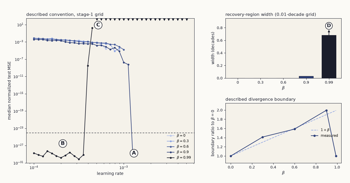
Figure 1. The described convention’s momentum recovery as a function of \(\beta\). Left: median normalized test MSE over three repetitions on the stage-1 grid; the dashed line is the frozen recovery threshold \(10^{-24}\). A — the \(\beta=0.9\) recovery at the last stable grid point. B — the \(\beta=0.99\) low-rate plateau on the error floor. C — the overflow row collects rates whose finite error exceeds \(10^{2}\) and rates that diverged. Upper right: refined recovery-region widths; D — the \(\beta=0.99\) region extends below its refinement window, so its bar is a lower bound. Lower right: the described divergence boundary relative to \(\beta=0\) against the \(1+\beta\) prediction.
Discussion
Overall verdict: falsified, as registered. The registered hypothesis had two clauses, and the second fired the falsifier: at \(\beta=0.6\) the described convention reaches the floor at no tested rate, its best median error 1.69×10⁻⁵ against the official convention’s best 8.55×10⁻²⁸ at the same \(\beta\). The first clause survived only in the letter — the count sequence 0, 0, 0, 1, 12 is nondecreasing — but a sequence that is zero, zero, zero before anything happens is not the monotone widening the hypothesis described, and the frozen decision rule says so.
What the curve actually does is more useful than what was predicted. Momentum’s rescue of the described convention is bimodal. At \(\beta=0.9\) it is the knife-edge the July note suspected: a single stage-1 point, 0.03 decades wide at refinement, pressed against the divergence boundary — a grid search at \(0.05\)-decade resolution finds it by luck. At \(\beta=0.99\) the rescue is real and wide, at least 0.68 decades and uniform across repetitions, but it sits at the bottom of the rate range rather than riding the boundary, and the boundary itself no longer follows the heavy-ball rule: after tracking \(1+\beta\) within a grid step through \(\beta=0.9\), it falls back to the plain-SGD value, and the region between the plateau and the boundary is a band of explosive but finite errors reaching 7.55×10⁷¹. A practitioner running a learning-rate search near \(\beta=1\) on this parameterization will see astronomically large finite losses that are not overflow, and a floor that is reachable at small rates — a different hazard map than the one the \(1+\beta\) rule draws, not an absence of one. If this bimodal structure is already characterized somewhere in the heavy-ball literature, that reference is exactly what we would like to be sent.
On mechanism we can offer a reading, not a measurement. The quadratic heavy-ball bound \(2(1+\beta)/L\) assumes a fixed curvature and a quadratic mode; the boundary’s collapse between \(\beta=0.9\) and \(\beta=0.99\) says at least one of those premises fails there — either the relevant curvature moves with \(\beta\), or the mode that diverges first at \(\beta=0.99\) is not the mode the bound describes. The velocity amplification \(1/(1-\beta)=100\) at \(\beta=0.99\) is the natural candidate for why the low-rate region trains at all: a hundred-fold amplification of persistent gradients is large enough to move the \(\omega_0^2\)-handicapped hidden stack at rates where plain SGD cannot. Both readings are testable and neither is tested here; the Conclusion queues the test.
Limits. One task, whose exactly linear cross-correlation lets the affine branch carry the fit; one architecture; three repetitions; full-batch heavy-ball without a Nesterov arm; a \(10^{-24}\) threshold whose sensitivity checks at \(10^{-20}\) and \(10^{-28}\) change nothing here but might elsewhere; a \(\beta=0.99\) plateau whose lower edge is unmeasured below \(7.9\times10^{-5}\); a different machine than the earlier notes, which moves roundoff-scale floor values; and a reimplementation of an unreleased specification, which bounds every claim to the written K1 setup.
Conclusion
The recovery-region question now has its curve, and it is not the predicted one: the set of rates at which momentum lets the described convention reach the official floor is empty through \(\beta=0.6\), a 0.03-decade knife-edge at \(\beta=0.9\), and a censored 0.68-decade plateau at \(\beta=0.99\) whose divergence boundary has fallen back to the plain-SGD value. Two experiments follow. First, the boundary collapse: track the top curvature along the training trajectory at \(\beta=0.9\) and \(\beta=0.99\) and test whether the quadratic heavy-ball bound fails there because \(L\) moves or because the first-diverging mode changes — the mechanism measurement this note declined to assert. Second, the plateau’s lower edge: extend the grid below \(7.9\times10^{-5}\) at \(\beta=0.99\) until the described convention leaves the floor, turning this note’s lower bound into a width. Both go on the shelf.