Why some atoms cost more than their neighbors

This note asks why chemically related and neighboring atoms can take different amounts of computation under the same electronic-structure protocol. The answer has two parts: the chosen model decides how much of the atom the computer must represent, and the iterative solver decides how many times it must work on that representation. A fixed panel of halogens, alkaline earths, transition metals, and the Kr/Rb boundary makes those two parts visible without pretending to price the whole periodic table.

An atom becomes matrices

Atomic number enters the nuclear potential, but the dominant numerical work is not proportional to atomic number alone. An electronic-structure program expands each molecular orbital in a finite set of basis functions,

\[ \phi_i(\mathbf r)=\sum_{\mu=1}^{N_{\mathrm{bf}}}C_{\mu i}\chi_\mu(\mathbf r), \]

then solves a matrix equation of dimension \(N_{\mathrm{bf}}\),

\[ \mathbf F[\mathbf P]\mathbf C =\mathbf S\mathbf C\boldsymbol\varepsilon. \]

The Fock matrix \(\mathbf F\) depends on the density \(\mathbf P\) built from the orbitals in \(\mathbf C\), so the program rebuilds and solves until input and output densities agree. That loop is the self-consistent field (SCF). Larger bases make those matrices and the work that constructs them larger; finite-basis SCF is an iterative numerical problem, not a lookup table for an element.^1,2

A useful bookkeeping approximation is

\[ T_{\mathrm{SCF}}\approx n_{\mathrm{iter}} \left[T_{\mathrm{build}}(N_e,N_{\mathrm{bf}}) +T_{\mathrm{solve}}(N_{\mathrm{bf}})\right]+T_{\mathrm{fixed}}. \]

It is not a fitted timing law. It simply separates work per cycle from number of cycles, while admitting fixed overhead. For the two survey repeats here, the plotted time is \(\widetilde T=\operatorname{median}(T_0,T_1)=(T_0+T_1)/2\). The survey compares unrestricted Hartree–Fock (UHF), which gives the two spin channels separate orbitals, with unrestricted Kohn–Sham PBE (UKS/PBE), a density-functional calculation with the same finite basis. Both close an SCF loop. Figure 1 places the representation counts and their timings side by side.

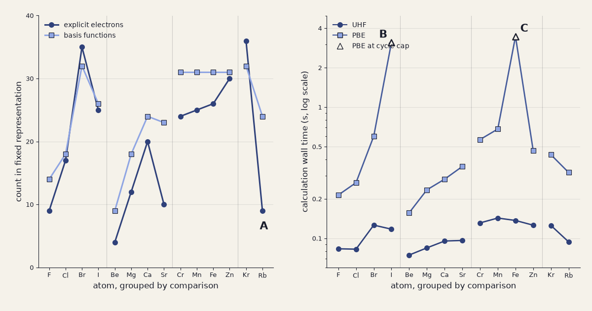
Two-panel plot of fourteen atoms grouped as halogens, alkaline earths, transition-metal comparisons, and the krypton-rubidium boundary. The left panel compares explicit electrons with basis functions. The right compares UHF and PBE wall time on a logarithmic axis, with iodine and iron marked as PBE attempts that reached the cycle cap.

Figure 1. The left panel follows explicit-electron and spherical def2-SVP basis-function counts; the right follows median two-repeat UHF and PBE calculation time on a logarithmic axis. A marks the Kr/Rb effective-core seam. B and C mark I/PBE and Fe/PBE reaching the fixed 80-cycle cap; their elapsed times are censored failed attempts, not completed timings.

The core can disappear from the calculation

For an all-electron calculation, \(N_e=Z\). With an effective core potential (ECP),

\[ N_e^{\mathrm{explicit}}=Z-N_{\mathrm{core}}^{\mathrm{ECP}}. \]

The def2-SVP setup used here is all-electron through Kr, then uses a 28-electron core for Rb, Sr, and I.³ Crossing from Kr to Rb therefore raised \(Z\) from 36 to 37 while the represented electron count fell from 36 to 9 and the basis count fell from 32 to 24. Among the repeated survey methods, Rb took 25.1% less wall time at UHF and 26.8% less at PBE. Its single second-order M{ø}ller–Plesset (MP2) attempt took 27.7% less than Kr’s. The largest repeat-to-repeat range among successful survey pairs, defined as \((T_{\max}-T_{\min})/\widetilde T\), was 8.2%.

That reversal is not a claim that Rb is intrinsically cheaper than Kr. It says the code was asked to represent less of Rb explicitly under this basis/ECP choice. “Cost of an element” already contains a modeling decision before the solver begins.

Equal-sized matrices can take unequal paths

Representation size is not enough. Cr, Mn, Fe, and Zn each used 31 basis functions, but their PBE SCF paths ended at 9, 12, 80, and 6 cycles. Each of the 2 Fe/PBE attempts reached the cap without convergence. Each of the 2 I/PBE attempts did the same at 80 cycles.

SCF equations can possess several stationary solutions and can oscillate or stall, especially around small gaps and competing occupations.² Those facts explain why iteration count is a separate cost axis; they do not diagnose these two failures. UHF converged for both atoms, and the other ECP atoms converged under PBE. The narrow statement earned here is that these particular UKS/PBE calculations did not settle under the fixed initial guess, grid, threshold, and cycle cap.

A method name is not a stopwatch

PBE, MP2, and CCSD(T) are different approximation families, not consecutive rungs of one runtime ladder. PBE is a generalized-gradient density functional; MP2 is second-order many-electron perturbation theory; CCSD(T) adds a perturbative triples correction to coupled cluster with singles and doubles.^4–6

On the 4 light atoms given all four methods, CCSD(T) took 1.66–2.65 times the UHF wall time. Yet PBE took longer than CCSD(T) in 4 of those cases. That does not make PBE the more expensive method in general. At these sizes, the reversal could reflect grid work, fixed setup, or solver details; this run did not separate them. The calculation did not earn a scaling exponent, so none is fitted.

Reproducibility

The fixed panel contained 14 neutral atoms and 70 fresh, single-threaded attempts. UHF and UKS/PBE ran twice for every atom; UMP2 ran once for the halogens, alkaline earths, and Kr/Rb; UCCSD(T) ran once for F, Cl, Be, and Mg. Of those attempts, 66 returned ok and 4 reached the SCF cap. Each calculation used spherical def2-SVP functions, the nominal Hund-rule spin, no point-group symmetry or density fitting, a minao guess, and an 80-cycle SCF limit.

The run used CPython 3.12.3, PySCF 2.13.1, NumPy 2.5.1, and one Intel i7-1165G7 laptop core per child process. PySCF supplied the UHF, UKS, UMP2, and UCCSD(T) implementations.⁷ The earlier Hartree–Fock note follows one SCF loop in more detail.

sweep.py embeds the atomic specifications; there is no external computational dataset. The append-only results/runs.jsonl is the canonical output. analyze.py validates the fixed job matrix, writes results/summary.json, and regenerates Figure 1; generate-metrics.mjs projects the typed values used in this post. Running python3 research/periodic-compute-cost/analyze.py --check under Matplotlib 3.11.1 reproduces the committed summary and figure. Running node research/periodic-compute-cost/generate-metrics.mjs --check and node scripts/verify-metrics.mjs checks the projection and its source fingerprints. That makes the note analysis-reproducible from its committed outputs; it does not make subsecond laptop timings hardware-independent.

Where the model stops

This probe times one finite-basis energy calculation, not “understanding an element” in the spectroscopic sense. The nominal spin does not establish the ground atomic term, the ECP seam changes the model as well as the atom, and no all-electron Rb control isolates the ECP’s causal share. The correlated-method timings are single attempts on four tiny atoms. The PBE failures were neither retried nor diagnosed with occupation or stability analyses, so they mean only that the frozen protocol failed to converge.

A controlled next step would hold the atom fixed while changing its core treatment, or hold the representation fixed while auditing alternative SCF occupations. This note stops before either expansion. Its narrower answer is enough: atomic number does not set computational cost by itself. The representation fixes the size of each numerical problem; the solver path fixes how many times that problem is paid for.

References

Helgaker, T.; Jørgensen, P.; Olsen, J. Molecular Electronic-Structure Theory; John Wiley & Sons: Chichester, 2000.

Lehtola, S.; Blockhuys, F.; Van Alsenoy, C. An Overview of Self-Consistent Field Calculations Within Finite Basis Sets. Molecules 2020, 25 (5), 1218. https://doi.org/10.3390/molecules25051218.

Weigend, F.; Ahlrichs, R. Balanced Basis Sets of Split Valence, Triple Zeta Valence and Quadruple Zeta Valence Quality for h to Rn: Design and Assessment of Accuracy. Physical Chemistry Chemical Physics 2005, 7 (18), 3297–3305. https://doi.org/10.1039/b508541a.

Perdew, J. P.; Burke, K.; Ernzerhof, M. Generalized Gradient Approximation Made Simple. Physical Review Letters 1996, 77 (18), 3865–3868. https://doi.org/10.1103/PhysRevLett.77.3865.

Møller, Chr.; Plesset, M. S. Note on an Approximation Treatment for Many-Electron Systems. Physical Review 1934, 46 (7), 618–622. https://doi.org/10.1103/PhysRev.46.618.

Raghavachari, K.; Trucks, G. W.; Pople, J. A.; Head-Gordon, M. A Fifth-Order Perturbation Comparison of Electron Correlation Theories. Chemical Physics Letters 1989, 157 (6), 479–483. https://doi.org/10.1016/S0009-2614(89)87395-6.

Sun, Q.; Zhang, X.; Banerjee, S.; Bao, P.; Barbry, M.; Blunt, N. S.; Bogdanov, N. A.; Booth, G. H.; Chen, J.; Cui, Z.-H.; Eriksen, J. J.; Gao, Y.; Guo, S.; Hermann, J.; Hermes, M. R.; Koh, K.; Koval, P.; Lehtola, S.; Li, Z.; Liu, J.; Mardirossian, N.; McClain, J. D.; Motta, M.; Mussard, B.; Pham, H. Q.; Pulkin, A.; Purwanto, W.; Robinson, P. J.; Ronca, E.; Sayfutyarova, E. R.; Scheurer, M.; Schurkus, H. F.; Smith, J. E. T.; Sun, C.; Sun, S.-N.; Upadhyay, S.; Wagner, L. K.; Wang, X.; White, A.; Whitfield, J. D.; Williamson, M. J.; Wouters, S.; Yang, J.; Yu, J. M.; Zhu, T.; Berkelbach, T. C.; Sharma, S.; Sokolov, A. Yu.; Chan, G. K.-L. Recent Developments in the PySCF Program Package. The Journal of Chemical Physics 2020, 153 (2), 024109. https://doi.org/10.1063/5.0006074.