
What a chord looks like: sound waves, harmonics, and Fourier transforms
A microphone records a chord as one changing voltage; in the air, it is one changing pressure. It does not arrive with separate labels for root, third, and fifth. The explanatory question for this note is therefore concrete: what physical signal does a chord make, and what does a Fourier transform reveal about it? We will build the answer from one sine wave, add the overtones that make a musical tone, sum three tones into a chord, use beats and frequency ratios to connect the spectrum back to music theory, and finally ask why that addition rule worked in the first place. This is the acoustical floor beneath harmony, not a claim that the floor is the whole building.1
One signal, two views
At a fixed point in space, sound can be represented by the departure of air pressure from its resting value. The simplest periodic model is
\[ p(t)=A\sin(2\pi f t+\phi), \]
where \(A\) is amplitude, \(f\) is frequency in cycles per second, and \(\phi\) says where in the cycle the wave begins. A frequency of \(440\ \mathrm{Hz}\) completes 440 cycles each second. Its period is the reciprocal, \(T=1/f=2.273\ \mathrm{ms}\).
The left side of Figure 1 shows ten milliseconds of that signal. The right side shows the magnitude of its discrete Fourier transform. Time has not disappeared; the transform has asked a different question of the same samples: how much of each sinusoidal frequency is required to reconstruct them? For this deliberately simple signal, nearly all the magnitude is concentrated at \(440\ \mathrm{Hz}\).
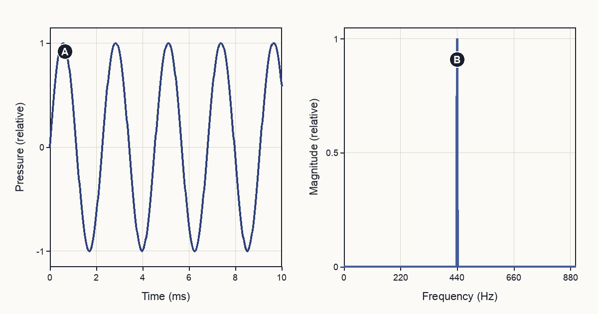
Figure 1. One synthetic A4 in two coordinate systems: A marks the repeating pressure signal in time, and B marks its concentrated Fourier magnitude at \(440\ \mathrm{Hz}\).
For sampled data \(x_n\), the transform used here is
\[ X_k=\sum_{n=0}^{N-1}x_n w_n \exp\!\left(-\frac{2\pi i k n}{N}\right), \]
with a Hann window \(w_n\). A finite observation cuts a signal off; the window softens that cut so the artificial edge contributes less spectral leakage. Window choice changes the width and sidelobes of spectral peaks, which is why a Fourier plot is a measurement with settings rather than a transparent view into the signal.2 The figures plot \(|X_k|\), the magnitude. They discard the complex phase of \(X_k\), so even this frequency view does not contain every visible fact about the time waveform.
A musical note is already a stack
A tuning fork approaches the sine-wave ideal. A string, reed, lip, air column, or instrument body generally does not. Its allowed modes and the way it is driven produce a fundamental together with partials. For many pitched instruments those partials lie approximately at integer multiples of the fundamental,
\[ p(t)=\sum_{m=1}^{M} A_m\sin(2\pi m f_0t+\phi_m). \]
The synthetic tone in Figure 2 uses eight such harmonics with \(A_m=m^{-1.2}\). The exponent is a convenient roll-off, not a model of a particular instrument. It is enough to make the point: the time waveform becomes sharper and less sinusoidal as the spectrum becomes a ladder at \(f_0,2f_0,3f_0,\ldots\). Real instruments add frequency-dependent radiation, inharmonicity, noise, and a changing attack and decay; instrument acoustics is largely the study of where those components come from.3
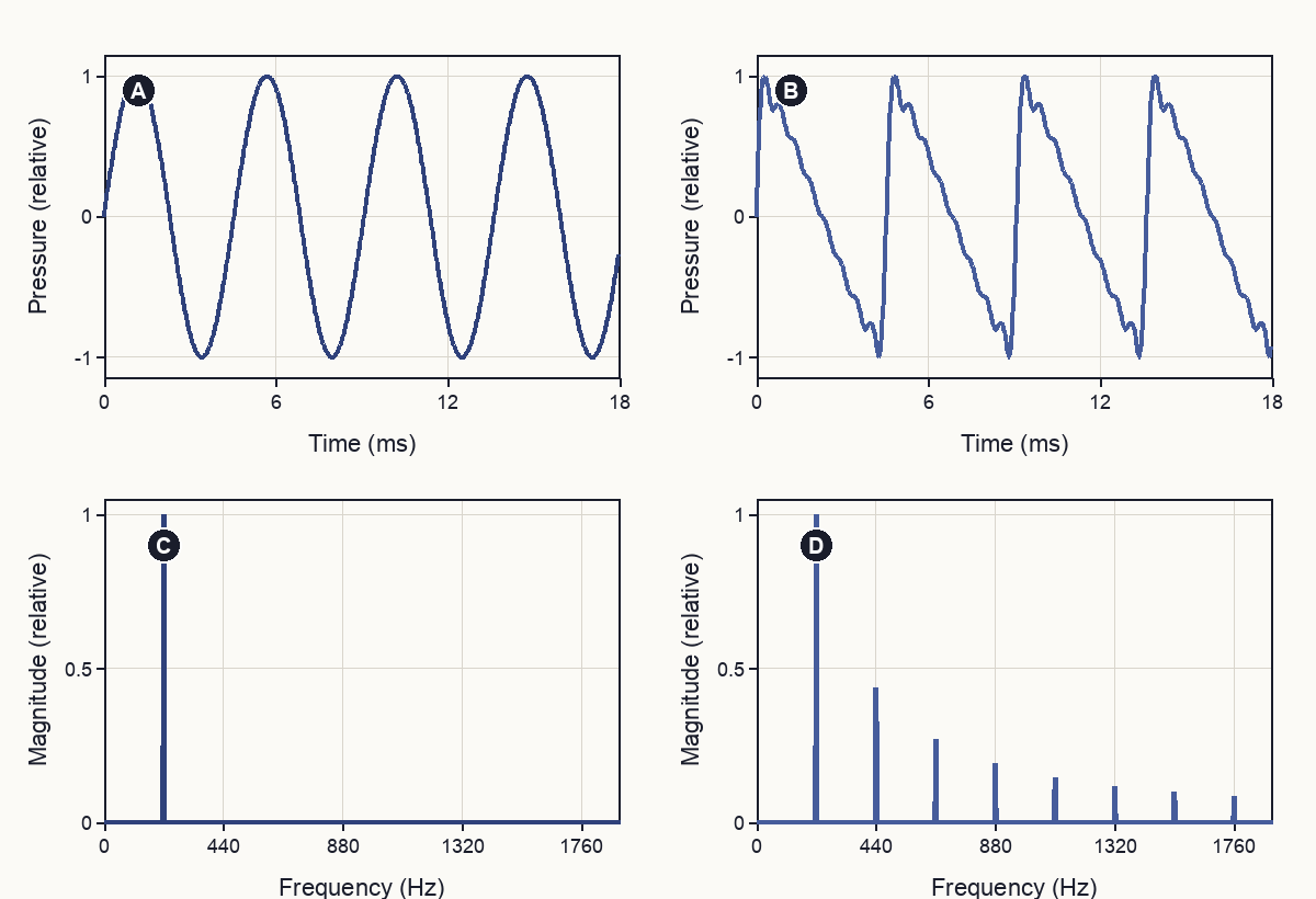
Figure 2. A pure tone and an additive harmonic tone at the same fundamental: A is the sine waveform, B is the waveform formed by eight partials, C is the sine’s single Fourier peak, and D is the harmonic ladder.
This is part of what physicists mean by timbre, but only part. Two tones can share a long-time magnitude spectrum and differ in phase, attack, decay, noise, or spectral evolution. Timbre belongs to the entire time-varying sound, while a single magnitude spectrum is one projection of it.4
A chord is addition
Twelve-tone equal temperament assigns a frequency \(n\) semitones away from A4 by
\[ f(n)=440\times 2^{n/12}\ \mathrm{Hz}. \]
For C4, E4, and G4 this gives \(261.626\), \(329.628\), and \(391.995\ \mathrm{Hz}\). An idealized C-major chord is simply their sum,
\[ p_{\mathrm{C}}(t)= \sin(2\pi f_{\mathrm{C4}}t)+ \sin(2\pi f_{\mathrm{E4}}t)+ \sin(2\pi f_{\mathrm{G4}}t). \]
The left side of Figure 3 keeps the three components apart long enough to show the bookkeeping, then gives their sum on the bottom line. The sum looks less regular because the three cycles continually move into and out of alignment. The spectrum on the right was made from a richer version of the same chord, with eight harmonics added to each note. What is tangled in time becomes an orderly collection of fundamentals and partials in frequency.
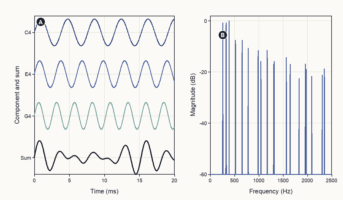
Figure 3. Superposition builds a C-major chord: A marks the three pure components above their summed pressure wave, while B marks the fundamental region of the harmonically enriched chord’s Fourier spectrum.
Audio 1 uses the same three fundamentals as Figure 3 without upper partials or attack transients, so it sounds organ-like. Audio 2 adds eight-partial ladders; it is still plainly synthetic, but the added harmonics change its color.
Audio 1. A synthetic C-major chord made from pure C4, E4, and G4 sine waves with a fixed attack and decay.
Audio 2. The same C-major fundamentals with eight harmonic partials per note, weighted as \(m^{-1.2}\).
Major and minor move one ladder
C minor changes E4 to E-flat4, \(311.127\ \mathrm{Hz}\). In a score that is one lowered note. In a spectrum it moves the fundamental by \(18.501\ \mathrm{Hz}\) and moves every one of that note’s partials with it. Figure 4 shows both harmonic-rich chords on the same axes. The C and G ladders stay fixed; the middle ladder is displaced.
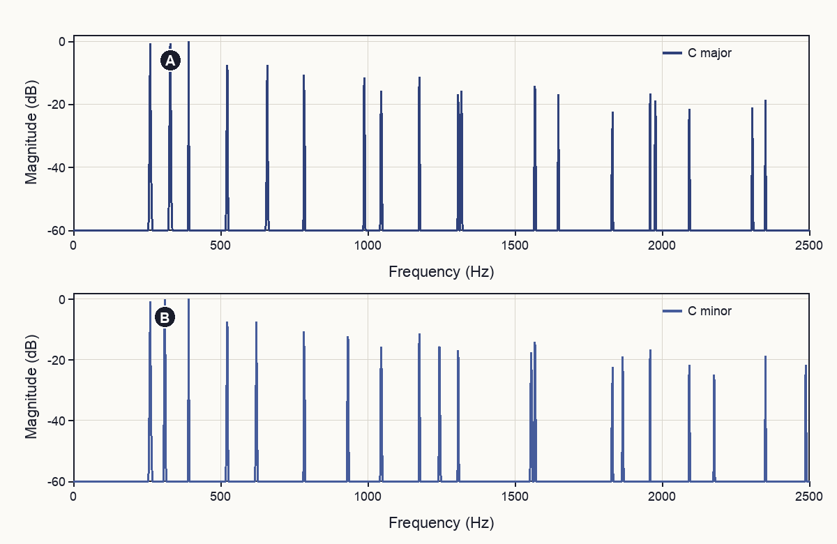
Figure 4. Equal-tempered C major and C minor as harmonic spectra: A marks the E4 fundamental in the major chord, and B marks its displacement to E-flat4 in the minor chord.
The plot supplies a physical description of the change, not the musical meaning of “major” and “minor.” It does not identify a tonic, establish harmonic function, or say how the chord behaves in a progression. The waveform contains frequencies; the grammar that organizes them operates at another level.
Beats put a frequency difference into time
When two nearby frequencies are added, a trigonometric identity separates a rapid carrier from a slow envelope:
\[ \sin(2\pi f_1t)+\sin(2\pi f_2t) =2\sin\!\left(2\pi\frac{f_1+f_2}{2}t\right) \cos\!\left(2\pi\frac{f_1-f_2}{2}t\right). \]
For \(f_1=440\ \mathrm{Hz}\) and \(f_2=442\ \mathrm{Hz}\), the fast part runs at \(441\ \mathrm{Hz}\) while the absolute amplitude rises and falls twice per second. Figure 5 makes both descriptions visible: the left plot is densely filled by the carrier but bounded by the slow envelope; the right plot resolves the two frequencies that create it.
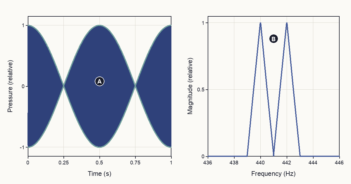
Figure 5. Two close tones in time and frequency: A marks a cancellation in the two-beat-per-second amplitude envelope, and B marks the pair of Fourier peaks at \(440\) and \(442\ \mathrm{Hz}\).
Audio 3 makes the slow envelope from Figure 5 audible.
Audio 3. Pure sine tones at \(440\) and \(442\ \mathrm{Hz}\) combine so their amplitude rises and falls twice per second.
Why superposition worked
Everything so far has treated the sound path as linear. In a linear system, doubling a pressure signal doubles the response, and adding two signals adds their responses. That is why the harmonic ladders in Figure 3 can coexist without manufacturing extra frequencies. At ordinary listening levels this is an excellent approximation for propagation through air and for audio equipment operating within its intended range. It is still an approximation.
A compact way to mark its boundary is a memoryless polynomial,
\[ y(t)=x(t)+\alpha x^2(t)+\beta x^3(t). \]
The first term is linear, \(\alpha x^2\) is a quadratic response, and \(\beta x^3\) is a cubic response. “Memoryless” means that the output at each instant depends only on the input at that instant. This is a demonstration of frequency mixing, not a model fitted to a particular instrument, room, ear, or listener.
For two pure inputs,
\[ x(t)=\sin a+\sin b, \qquad a=2\pi f_1t,\quad b=2\pi f_2t, \]
the quadratic term can be reconstructed directly:
\[ x^2(t)= 1-\frac{1}{2}\cos(2a)-\frac{1}{2}\cos(2b) +\cos(a-b)-\cos(a+b). \]
Besides a constant component, it contains \(2f_1\), \(2f_2\), \(|f_2-f_1|\), and \(f_1+f_2\). The constant is omitted from the figure and audio because it is a static offset rather than a sustained audible frequency. The cubic term is
\[ \begin{aligned} x^3(t)={}& \frac{9}{4}\left(\sin a+\sin b\right) -\frac{1}{4}\left(\sin 3a+\sin 3b\right)\\ &+\frac{3}{4}\left[\sin(2a-b)+\sin(2b-a)\right]\\ &-\frac{3}{4}\left[\sin(2a+b)+\sin(a+2b)\right]. \end{aligned} \]
It strengthens the two inputs and adds \(3f_1\), \(3f_2\), \(2f_1\pm f_2\), and \(2f_2\pm f_1\). Order describes the power of the input in the response law, not the number of a resulting harmonic: a quadratic response is not merely “the second harmonic,” nor is a cubic response merely “the third harmonic.”
This exposes an easily missed distinction in Figure 5. Linear addition makes the amplitude of \(440\) and \(442\ \mathrm{Hz}\) rise and fall twice per second, but their spectrum contains no \(2\ \mathrm{Hz}\) line. A quadratic response has the explicit term \(\cos(a-b)\) and therefore creates a component at the difference frequency. The difference frequency exists in the spectrum only if something nonlinear puts it there.
Figure 6 applies the same calculation to equal-tempered C4 and E4, \(f_1=261.626\ \mathrm{Hz}\) and \(f_2=329.628\ \mathrm{Hz}\). Panel A is the clean input. Panel B places the four nonconstant quadratic products at \(68.002\), \(523.251\), \(591.253\), and \(659.255\ \mathrm{Hz}\). Panel C removes the strengthened C4 and E4 components and places the six new cubic products at \(193.624\), \(397.630\), \(784.877\), \(852.879\), \(920.881\), and \(988.883\ \mathrm{Hz}\).
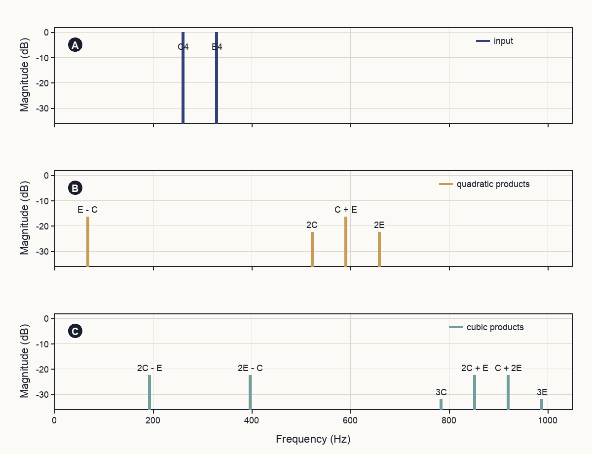
Figure 6. Two-tone intermodulation: A contains only the C4 and E4 input frequencies, B isolates the nonconstant quadratic products, and C isolates the new cubic products after removing the strengthened inputs. All three panels share an input-referenced decibel scale; the illustrative values \(\alpha=0.15\) and \(\beta=0.10\) make the product families visible but do not represent measured propagation through air.
Audio 4–6 isolate the same three layers. The two product layers are each raised to the same RMS level as the input after isolation. That magnification preserves relative amplitudes within each order while making otherwise faint components audible. Their playback loudness therefore demonstrates frequency content, not real-world nonlinear strength. The \(68\ \mathrm{Hz}\) quadratic product may require headphones or speakers capable of reproducing low bass.
Audio 4. Equal-amplitude pure tones at C4 and E4, containing only \(261.626\) and \(329.628\ \mathrm{Hz}\) before the shared attack and decay.
Audio 5. The four isolated quadratic products of the C4–E4 pair, with the constant component omitted and the remaining signal magnified as one layer.
Audio 6. The six isolated new cubic products of the C4–E4 pair, with the strengthened C4 and E4 components omitted and the remaining signal magnified as one layer.
The difference product also carries tuning information. If E is placed at a just \(5{:}4\) above the same C4, then \(f_E-f_C=f_C/4=65.406\ \mathrm{Hz}\), exactly C2. Equal temperament instead produces \(68.002\ \mathrm{Hz}\), which is \(67.4\) cents—about two-thirds of a semitone—above C2. The tuning compromise in the next section therefore appears not only in overlapping partials but in frequencies created by nonlinear mixing.
Real musical systems put nonlinearity in different places. Measurements of a trombone played fortissimo found wave steepening and shock formation in its bore, which the authors connected to the brightness of loud brass sound.5 Fletcher’s review describes nonlinear driving in sustained instruments and high-frequency energy transfer after strikes of gongs and cymbals.6 Kemp measured stimulated acoustic emissions from human ears and attributed the delayed response to a nonlinear mechanical mechanism probably located in the cochlea.7 The polynomial and audio above show the shared mixing mathematics. They do not establish how large these products are in any instrument or ear, or what a listener perceives.
Beating is one physical ingredient in acoustic roughness. With complex tones, each partial in one note can form a beating pair with each partial in another. Classic work connected the strongest roughness region to separations within a fraction of an auditory critical band, rather than to a frequency difference that is constant across the spectrum.8 That result is a bridge from acoustics into psychoacoustics, not a formula that ranks every chord in every musical setting.
Small ratios align partials
The familiar ratios attached to intervals now have a visible meaning. An octave at \(2{:}1\) makes every partial of the upper note coincide with an even-numbered partial of the lower note. A just perfect fifth at \(3{:}2\) makes the lower note’s third partial coincide with the upper note’s second:
\[ 3f_0=2\left(\frac{3}{2}f_0\right). \]
Equal temperament chooses a slightly different fifth, \(2^{7/12}=1.498307\) rather than \(1.5\). Above C4, the just G is \(392.438\ \mathrm{Hz}\) and the equal-tempered G is \(391.995\ \mathrm{Hz}\). Their fundamentals differ by only \(0.443\ \mathrm{Hz}\), but at the supposedly shared partial the separation doubles: \(3f_{\mathrm{C4}}\) and \(2f_{\mathrm{G4}}\) are \(0.886\ \mathrm{Hz}\) apart.
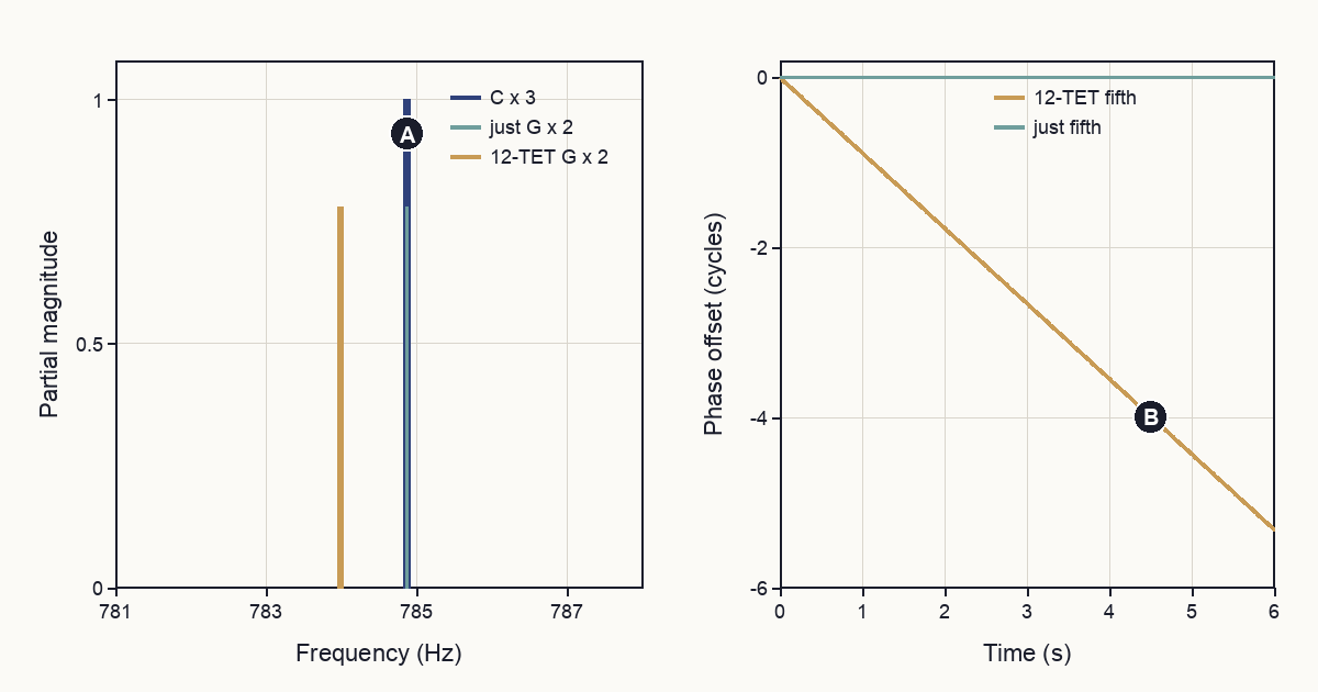
Figure 7. Harmonic alignment in a perfect fifth: A marks the exact coincidence of \(3f_{\mathrm{C4}}\) and twice the justly tuned G4 beside the slightly lower equal-tempered partial, while B marks the equal-tempered pair’s accumulated phase slip; the just pair remains at zero.
Equal temperament has not made the fifth “wrong.” It has exchanged exact local ratios for twelve equal logarithmic steps, so every key receives the same interval pattern. Figure 7 shows the physical price of that design choice. The musical value of the trade depends on the tuning system, instruments, ensemble, and repertoire.
How the figures were made
Every signal, spectrum, image, and audio clip in this note was generated on an arm64 Mac with CPython 3.13.12, NumPy 2.4.4, and Pillow 12.2.0. Signals were sampled at \(44{,}100\ \mathrm{Hz}\). Figures 1–5 and 7 use NumPy’s real discrete Fourier transform after a Hann window and normalize spectra to their largest magnitude. The harmonic demonstrations use eight sine partials with amplitudes \(m^{-1.2}\); phases are zero, and there is no noise or random input.
Figure 6 instead plots the exact line components in the displayed polynomial, with \(\alpha=0.15\) and \(\beta=0.10\), relative to unit-amplitude inputs. Audio 4–6 use the same equal-tempered C4 and E4. Their linear, nonconstant quadratic, and new cubic layers are constructed from the written identities before one common attack-and-decay envelope is applied. Each complete layer is then set to an RMS amplitude of \(0.17\), subject to a peak ceiling of \(0.88\); components within a layer never receive separate gain. The highest generated frequency is \(988.883\ \mathrm{Hz}\), far below the \(22{,}050\ \mathrm{Hz}\) Nyquist limit. No recordings, external datasets, random inputs, or living subjects were used.
The complete generator is available as a single Python script. It recreates all seven PNG figures and the six WAV files from constants printed in the source.
Where the physical picture stops
A Fourier transform can expose frequency, harmonicity, beating, and the spectral change caused by moving one note. It cannot read a Roman numeral from a waveform. It does not know which pitch is the root, whether a chord is stable or tense in context, where a phrase is going, or why the same sonority can carry different meanings in different musical systems.
Even at the acoustical level, these demonstrations are deliberately thin. Real notes change from millisecond to millisecond; rooms add reflections; instruments deviate from perfect harmonicity; performers tune and voice notes dynamically; and ears do not perform an unmodified FFT. The polynomial demonstration proves where ideal quadratic and cubic terms place frequencies, but its magnified audio does not measure nonlinear air, an instrument, a cochlea, or perception; no listening experiment was performed. The spectrum is therefore best used as one well-defined view. It explains how several notes can occupy one pressure wave, how their partials meet, and how a nonlinear response can add new components. Music theory begins where those physical facts are organized across time.