
Where Coulomb subtraction helps a neural potential fit
Abstract
Rana and co-workers introduced a physically appealing way to fit molecular potential energy curves: subtract the exact nuclear repulsion, fit the electronic energy, and restore the exact term afterward. I use the one-electron H\(_2^+\) curve to ask where that decomposition helps a small neural network, rather than whether it works in general. A 401-point UHF/aug-cc-pV5Z curve from \(0.15\) to \(20\,a_0\) was refit at eight lower-distance cutoffs with matched folds, initial weights, and training budgets. When the domain starts at \(0.15\,a_0\), the median seed-wise out-of-fold RMSEs are 26,270 cm\(^{-1}\) for a direct total-energy fit and 569 cm\(^{-1}\) after Coulomb subtraction; the median of five paired A/B ratios is 44.9. That paired ratio falls to 5.21 at \(0.7\,a_0\), 1.19 at \(1.5\,a_0\), 0.954 at \(2.0\,a_0\), and 0.102 at \(3.0\,a_0\). Seven sensitivity configurations spanning input, scaling, width, sample count, optimization, and basis put the transition between \(0.7\) and \(2.0\,a_0\), with its exact location dependent on representation and metric. For this small H\(_2^+\) network, Coulomb subtraction is a strong conditioning choice when one fit must cover the repulsive wall; on a domain beginning beyond the minimum, the direct total potential is the simpler target.
Introduction
At fixed nuclei, a molecular potential separates into an electronic energy and a nuclear-repulsion term,
\[ V(\mathbf R) = E_{\mathrm{el}}(\mathbf R) + V_{\mathrm{NN}}(\mathbf R), \qquad V_{\mathrm{NN}} = \sum_{A<B}\frac{Z_AZ_B}{R_{AB}}. \]
Rana and co-workers turned that identity into a useful fitting strategy. Their Scheme A fits \(V\) directly. Their Scheme B fits \(E_{\mathrm{el}}\) and adds the known \(V_{\mathrm{NN}}\) back to every prediction. The decomposition builds the divergent short-range physics into the model instead of asking a finite neural network to learn it from samples.1
That idea raises a practical question the original study did not need to isolate: how much of the fitted distance range has to contain close nuclear approaches before subtraction earns its keep? A residual can be physically well chosen without being uniformly easier to approximate on every restricted domain. Mapping that dependence extends the decomposition by identifying the fit domains where it provides the largest numerical benefit.
H\(_2^+\) makes the question unusually clean. It has one coordinate, one electron, and an exact nuclear term \(V_{\mathrm{NN}}(R)=1/R\). Scheme B therefore changes only the target seen by the network; it introduces no second electronic-structure calculation and no fitted long-range correction. Successively removing the shortest distances turns the question into a controlled scan from the repulsive wall, through the equilibrium well, and into the dissociation tail. The one-electron choice also removes the correlation question that enters the corresponding water calculation.
Hypothesis. The benefit of Scheme B is concentrated at short distance, where \(1/R\) has its largest curvature, so the paired median ratio \(\operatorname{RMSE}(A)/\operatorname{RMSE}(B)\) will move toward 1 as the shortest geometries are removed. Falsifier. The hypothesis is rejected if the median ratio remains at least 2, without a downward trend, after every point below \(R=1.5\,a_0\) is removed. I would publish that outcome too: it would give the residual a broader useful range than the short-range argument predicts.
Computational Methods
The electronic-structure and neural calculations ran on a 10-core Apple M1 Pro MacBook Pro with 32 GB of memory, using arm64 macOS 26.5.2, CPython 3.14.6, NumPy 2.5.0, Psi4 1.11, and QCElemental 0.50.4. Psi4 supplied the electronic-structure energies.2 Final tabulation and figure generation used CPython 3.14.4, NumPy 2.3.4, Matplotlib 3.10.7, and Pillow 12.2.0; that step reads stored results and performs no refitting. The complete scripts, command ledger, frozen protocol, scan data, validation output, fit metrics, and summaries are in h2plus-coulomb-subtraction.tar.gz.
The electronic-structure data are for the ground electronic state of H\(_2^+\), with charge \(+1\) and multiplicity 2. The two protons were placed at \(z=\pm R/2\) in \(D_{2h}\) symmetry, without recentering or reorientation. I ran an independent core-Hamiltonian guess at each of 401 geometrically spaced distances from \(0.15\) to \(20\,a_0\). The production calculation used UHF with the aug-cc-pV5Z basis, density-fitted SCF, energy and density convergence thresholds of \(10^{-12}\) and \(10^{-10}\), two CPU threads, and a 4 GB memory limit. With one electron, Hartree–Fock has no electron-correlation approximation; its remaining electronic-structure error here is the finite orbital basis. The correlation-consistent and augmented basis families are described by Dunning and by Kendall, Dunning, and Harrison.3,4
At every geometry I recorded
\[ E_{\mathrm{el}} = V - V_{\mathrm{NN}}, \qquad V_{\mathrm{NN}}=1/R, \]
along with the one- and two-electron components, SCF iterations, AO and MO counts, smallest overlap eigenvalue, and point group. Representative points at \(R=0.15, 0.25, 0.5, 1, 2, 5, 10,\) and \(20\,a_0\) were repeated with aug-cc-pVTZ, aug-cc-pVQZ, direct-integral UHF/aug-cc-pV5Z, and ROHF/aug-cc-pV5Z. The \(R=2\,a_0\) electronic energy was also compared with the high-accuracy nonrelativistic value of Ishikawa, Nakashima, and Nakatsuji.5
For the primary neural experiment, I retained points with \(R\ge R_{\min}\) for each \(R_{\min}\) in \(\{0.15,0.25,0.40,0.70,1.00,1.50,2.00,3.00\}\,a_0\). Each cutoff defines a new fit and evaluation domain; it is not a pointwise label attached to an individual geometry. Five stratified folds were assigned once on the complete ordered grid and preserved across cutoffs. Within each consecutive five-point block, a permutation drawn with seed 70220 assigned one point to each fold. Every eligible point received one out-of-fold prediction.
Both schemes used a one-hidden-layer network with 15 tanh units and a linear readout, float64 arithmetic, Xavier-uniform weights, and zero biases. Raw \(R\) was standardized from the training-fold mean and standard deviation. Each target was standardized separately from its training-fold moments and returned to hartree before scoring. A Scheme B prediction was scored only after exact \(1/R\) restoration. Five initialization seeds (11, 29, 47, 71, 101) were used; within a fold and seed, Schemes A and B began from bit-identical parameters. This paired construction follows the same comparison discipline as the preceding neural-network experiment.
Optimization was full-batch Adam for a fixed 20,000 steps, with cosine learning-rate decay from \(10^{-3}\) to \(10^{-5}\) and no regularization. The checkpoint with the lowest training MSE was retained; test folds selected no checkpoint, seed, architecture, or hyperparameter. The primary outcome is pooled out-of-fold total-energy RMSE in cm\(^{-1}\) for each seed. The paired ratio \(A/B\) is above 1 when Scheme B has the smaller RMSE and below 1 when Scheme A does. MAE, maximum error, shortest-quintile RMSE, and a trapezoidal RMSE weighted uniformly in linear \(R\) were recorded as secondary outcomes.
The predeclared neural controls replaced raw \(R\) by \(\log R\), used Scheme A’s target standard deviation for both schemes, changed the hidden width to 10 or 20, and held the point count at 156 across cutoffs. The constant-count control retained rounded, evenly spaced eligible-grid indices at each cutoff. The predeclared electronic-structure control compared TZ, QZ, and 5Z energies at eight distances. Two follow-up sensitivity analyses, not predeclared controls, repeated the complete neural fit on the aug-cc-pVQZ curve and repeated both schemes together for 40,000 steps with learning rates from \(3\times10^{-4}\) to \(3\times10^{-6}\). These are fixed-capacity, fixed-budget comparisons, not estimates of either scheme’s converged approximation limit.
The article’s availability statement offers data on reasonable request; the public article and Supporting Information do not contain the energy grids, MATLAB code, split indices, preprocessing, or random seeds.1 I did not run the authors’ code or data. Every result below describes this independent H\(_2^+\) experiment, not a reproduction of their numerical tables.
Results
The 401-point production scan completed in 120.7 s. Every point converged in two SCF iterations with 160 AOs and 160 MOs. The smallest overlap eigenvalue was \(4.36\times10^{-9}\), and the basis rank remained 160 across the scan. Table 1 lists the electronic-structure checks.
Table 1. Numerical checks on the UHF/aug-cc-pV5Z production curve and the eight-point electronic-structure validation set.
| Check | Recorded value |
|---|---|
| \(\max|V-(E_{\mathrm{el}}+V_{\mathrm{NN}})|\) | \(2.22\times10^{-16}\ E_h\) |
| \(\max|V_{\mathrm{NN}}-1/R|\) | \(4.44\times10^{-15}\ E_h\) |
| maximum two-electron component | \(5.55\times10^{-16}\ E_h\) |
| maximum DF–direct difference | \(8.88\times10^{-15}\ E_h\) |
| maximum UHF–ROHF difference | \(1.51\times10^{-14}\ E_h\) |
| maximum aug-cc-pVQZ–aug-cc-pV5Z difference | \(6.35\times10^{-4}\ E_h\) |
| sampled minimum \((R,V)\) | \((2.00590\,a_0,-0.6026188\ E_h)\) |
| \(E_{\mathrm{el}}(2\,a_0)\); difference from high-accuracy value | \(-1.1026223\ E_h\); \(1.19\times10^{-5}\ E_h\) |
| \(V(20\,a_0)\) | \(-0.50000899\ E_h\) |
Figure 1 plots the two target curves and the equal-point out-of-fold RMSE ratios. The shaded range is the minimum to maximum of the seven raw-\(R\) configuration medians at each cutoff; it is not a confidence interval.
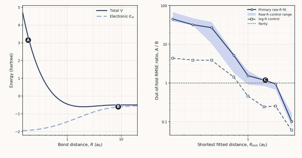
Figure 1. H\(_2^+\) energy targets and equal-point out-of-fold RMSE ratios. (A) marks the total-energy curve inside the short-range wall; (B) marks the electronic-energy curve at large \(R\); (C) marks RMSE parity near the primary curve between \(R_{\min}=1.5\) and \(2.0\,a_0\). The shaded area is the min–max range of configuration medians for seven raw-\(R\) settings, and \(R_{\min}\) is the lower bound of both the fitted and evaluated domain.
The primary fit returned the values in Table 2. The median ratio decreased from 44.938 at \(R_{\min}=0.15\,a_0\) to 1.187 at \(1.5\,a_0\), 0.954 at \(2.0\,a_0\), and 0.102 at \(3.0\,a_0\). All five paired seeds had ratios above 1 through \(R_{\min}=1.0\,a_0\); four did at \(1.5\,a_0\), two at \(2.0\,a_0\), and zero at \(3.0\,a_0\).
Table 2. Pooled out-of-fold total-energy RMSE for the primary 1–15–1 tanh network, with medians and ranges over five paired initialization seeds.
| \(R_{\min}\) (\(a_0\)) | points | median A RMSE (cm\(^{-1}\)) | median B RMSE (cm\(^{-1}\)) | median A/B [seed range] | B-favoring seeds |
|---|---|---|---|---|---|
| 0.15 | 401 | 26,269.89 | 568.94 | 44.938 [40.772, 51.427] | 5/5 |
| 0.25 | 359 | 8,440.15 | 264.15 | 31.952 [27.969, 36.411] | 5/5 |
| 0.40 | 320 | 2,480.69 | 90.56 | 26.856 [25.192, 31.954] | 5/5 |
| 0.70 | 275 | 650.46 | 125.50 | 5.214 [4.227, 7.303] | 5/5 |
| 1.00 | 245 | 191.46 | 124.50 | 1.546 [1.216, 2.116] | 5/5 |
| 1.50 | 212 | 115.21 | 93.39 | 1.187 [0.991, 1.655] | 4/5 |
| 2.00 | 189 | 57.56 | 61.29 | 0.954 [0.783, 1.110] | 2/5 |
| 3.00 | 156 | 2.88 | 31.21 | 0.102 [0.055, 0.123] | 0/5 |
Uniform-in-\(R\) weighting gave median A/B ratios of 27.354, 3.667, 1.213, 1.075, 0.895, and 0.100 at \(R_{\min}=0.15, 0.70, 1.00, 1.50, 2.00,\) and \(3.00\,a_0\), respectively. The primary checkpoint with the lowest recorded training loss occurred at step 20,000 in all 400 cutoff–fold–seed–scheme jobs.
Table 3 lists the median ratios at \(R_{\min}=0.70\)–\(3.00\,a_0\) for all eight fit configurations. Across all eight cutoffs, their 40 paired seed ratios per cutoff numbered 40 above 1 at \(R_{\min}=0.15\,a_0\), 39 at \(0.70\,a_0\), 26 at \(1.00\,a_0\), 24 at \(1.50\,a_0\), 9 at \(2.00\,a_0\), and 0 at \(3.00\,a_0\). All eight configuration medians were above 1 through \(0.70\,a_0\) and below 1 at \(2.00\) and \(3.00\,a_0\).
Table 3. Median equal-point out-of-fold RMSE ratio A/B over five paired seeds for each fit configuration and lower-domain cutoff.
| Configuration | 0.70 \(a_0\) | 1.00 \(a_0\) | 1.50 \(a_0\) | 2.00 \(a_0\) | 3.00 \(a_0\) |
|---|---|---|---|---|---|
| primary | 5.214 | 1.546 | 1.187 | 0.954 | 0.102 |
| common target scale | 3.735 | 0.992 | 1.006 | 0.791 | 0.076 |
| 10 hidden units | 1.822 | 0.899 | 0.843 | 0.895 | 0.106 |
| 20 hidden units | 4.213 | 1.443 | 1.029 | 0.787 | 0.086 |
| constant point count | 5.455 | 1.579 | 1.213 | 0.943 | 0.102 |
| 40,000 lower-rate steps | 5.754 | 2.088 | 1.033 | 0.675 | 0.166 |
| aug-cc-pVQZ curve | 5.269 | 1.541 | 1.182 | 0.951 | 0.107 |
| \(\log R\) input | 1.419 | 0.458 | 0.241 | 0.254 | 0.060 |
Discussion
Verdict: the hypothesis is supported. Its falsifier required the median ratio to remain at least 2 without a downward trend after removing every point below \(1.5\,a_0\). The primary ratio was 1.187 at that cutoff, 0.954 at \(2.0\,a_0\), and 0.102 at \(3.0\,a_0\). The broad result also persisted across the sensitivity configurations: by the primary equal-point metric, the median over seeds favored Scheme B for every configuration through \(0.7\,a_0\) and Scheme A for every configuration at \(2\) and \(3\,a_0\).
These results add a fit-domain map to the decomposition introduced by Rana and co-workers.1 When one small network must span close nuclear encounters and the bonding region, Scheme B is a strong conditioning device. At \(R_{\min}=0.15\,a_0\), the median paired error ratio is 44.9 under a matched training budget; the ratio of the two seed-wise median RMSEs is 46.2. The target curves provide a numerical explanation consistent with that separation: Scheme A’s target contains the \(1/R\) wall, while Scheme B assigns that wall to an exact analytic term and presents the network with the finite electronic curve. That is precisely the kind of structure a physics-informed residual is meant to remove.
The other side of Figure 1 matters just as much. Once the fitted domain begins at or beyond the equilibrium minimum, the total H\(_2^+\) potential is a shallow dissociation tail approaching \(-0.5\ E_h\). The electronic target is \(E_{\mathrm{el}}=V-1/R\), so it retains a much larger \(1/R\)-like tail even though adding \(1/R\) later reconstructs the correct total energy. At \(R_{\min}=3\,a_0\), the total target spans 0.0774 \(E_h\) and the electronic target spans 0.3604 \(E_h\); the direct network’s median RMSE is 2.88 cm\(^{-1}\) against 31.21 cm\(^{-1}\) for the residual network. Exact physics in the reconstruction does not guarantee that the residual is the easiest finite-network target on every restricted domain.
The \(\log R\) control sharpens that interpretation without turning it into a universal cutoff. A log coordinate already expands the compressed short-range region: its equal-point ratio at \(0.7\,a_0\) is 1.419 instead of the primary 5.214, and its uniform-in-\(R\)-weighted ratio there is 0.758. That result is consistent with input representation and Coulomb subtraction addressing partially overlapping parts of the same conditioning problem. Across metrics and representations, the stable statements are at the ends: for all eight configurations, the median ratio for each of the five recorded metrics favors Scheme B through \(R_{\min}=0.4\,a_0\) and Scheme A at \(3.0\,a_0\). The interval from roughly \(0.7\) to \(2.0\,a_0\) is a transition zone, not a molecular constant.
The controls argue against several alternative explanations. Holding the point count fixed follows the primary ratios closely, so shrinking sample count is unlikely to be the sole source of the trend. Common target scaling preserves the endpoint ordering, so separate standardization is unlikely to manufacture it. Widths of 10 and 20 units, a lower learning rate with twice the steps, and the independently generated aug-cc-pVQZ curve all retain the same endpoint ordering. At the five cutoffs in Table 3, the QZ ratios differ from the 5Z primary ratios by 0.055 or less; across all eight cutoffs, the largest difference is 0.969 at \(0.25\,a_0\).
There are four boundaries on the claim. First, each cutoff retrains and tests a new model on \(R\ge R_{\min}\); the scan maps a fit domain, not the pointwise value of subtraction at one geometry. Second, these five seeds are paired optimization repeats, not independent physical experiments, and the shaded configuration range in Figure 1 is descriptive rather than inferential. Third, the network is deliberately small and its absolute short-range errors are not a production-quality potential; nearly every job reached its lowest recorded training loss at the fixed-budget endpoint. Fourth, H\(_2^+\) is one-dimensional and one-electron. No result here establishes the same boundary for a polyatomic surface, force training, or a thermally sampled geometry distribution.
The shortest 37 aug-cc-pV5Z geometries also have overlap eigenvalues below \(10^{-8}\), although the basis rank stays fixed, direct and density-fitted SCF agree, and the QZ neural control returns the same pattern. I therefore treat \(0.15\,a_0\) as an extreme-compression stress test, not a chemically typical H–H distance. The practically useful result is not its exact 44.9 factor. It is the measured change of regime: subtracting known singular physics pays when the training distribution includes that physics, while a direct fit deserves its own benchmark when deployment is confined to the smooth tail.
Conclusion
The next design decision is no longer a blanket choice between total and electronic energies. It is a question about the support of the training distribution. For this H\(_2^+\) network, a domain that contains the repulsive wall strongly favors exact Coulomb subtraction; a domain that begins beyond the minimum favors the direct total potential; and the middle depends on coordinate, metric, and training details.
The next experiment is to add force labels to the same matched-cutoff scan. The energy contribution scales as \(1/R\), but its force scales as \(1/R^2\), so an energy-plus-force loss may extend Scheme B’s useful range. If the crossover does not move outward—or moves inward—the conditioning benefit is specific to energy fitting rather than strengthened by differentiation. That question now goes on the shelf.